[DL] MNIST_2.Deep Learning 구현

^{문성훈 강사님의 강의 내용을 기반으로 합니다.}

^{Tensorflow 1.X ver}

MNIST - Tensorflow로 Deep Learning 구현

지난 번에 Machine Learning으로 구현한 MNIST 문제를 Deep Learning으로 구현해 보자.

1. 주의

첫째, 여러 개의 weight 행렬과 bias를 설정한다. 딥러닝에서는 여러 layer를 만들어 신경망을 구현하고, 각 층에서 model을 구현하게 된다.

둘째, 적절한 수의 perceptron을 설정한다. layer가 너무 많으면 depth 문제로 시간이 오래 걸리고, 오히려 정확한 연산이 어려울 수 있다. 각 층별로 weight와 bias 설정에 주의하자.

셋째, layer 설정 시 weight, bias의 shape에 특히 유의하자. layer 간에도 맞아야 하고, W와 b 간에도 맞아야 한다.

넷째, 각 학습 layer 및 단계별로 data의 개수를 나누어 적절한 batch를 설정하고, epoch 역시 적절하게 설정하자.

뭔가 결국 다 custom을 잘 해야 하는 것 같은 건 착각인감..

2. 기본 딥러닝 모델 설정

2.1. 모듈 불러오기 및 데이터셋 준비

# module import
import tensorflow as tf
from tensorflow.examples.tutorials.mnist import input_data
import warnings

# load data
mnist = input_data.read_data_sets("./data/mnist", one_hot=True)

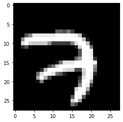
# check data
import matplotlib.pyplot as plt

plt.imshow(mnist.train.images[0].reshape(28, 28), cmap='gray')

2.2. 그래프 초기화, placeholder

tf.reset_default_graph()

# placeholder
X = tf.placeholder(shape=[None, 784], dtype=tf.float32)
Y = tf.placeholder(shape=[None, 10], dtype=tf.float32)

2.3. weight, bias

이 단계부터 달라진다. 문쌤은 3개의 layer를 설정하셨다. 물론 각 layer에서 구성하는 perceptron은 임의로 정한 수이다. 다음 layer로 넘겨 주어야 하므로, shape에 항상 유의하자. 제발.. 이제부터는 layer끼리 행렬곱이 들어간다.

# layer1 : X data 각각에 대해 256번 학습 진행.
W1 = tf.Variable(tf.random_normal([784, 256]), name='weight1')
b1 = tf.Variable(tf.random_normal([256]), name='bias1')
layer1 = tf.sigmoid(tf.matmul(X, W1) + b1)

# layer2 : 256번 학습한 걸 다시 돌려서 256번 학습 진행.
W2 = tf.Variable(tf.random_normal([256, 256]), name='weight2')
b2 = tf.Variable(tf.random_normal([256]), name='bias2')
layer2 = tf.sigmoid(tf.matmul(layer1, W2) + b2)

# layer3 : 최종적으로 10개의 라벨 값에 맞도록 학습 진행.
W3 = tf.Variable(tf.random_normal([256, 10]), name='bias3')
b3 = tf.Variable(tf.random_normal([10]), name='bias3')

2.4. hypothesis

로짓을 구하고, 활성화 함수를 설정한다.

logit = tf.matmul(layer2, W3) + b3
H = tf.nn.softmax(logit)

2.5. cost

cost = tf.reduce_mean(tf.nn.softmax_cross_entropy_with_logits_v2(logits=logit, labels=Y))

2.6. train

train = tf.train.GradientDescentOptimizer(learning_rate=0.1).minimize(cost)

2.7. session, 변수 초기화

sess = tf.Session()
sess.run(tf.global_variables_initializer())

2.8. 학습

이전과 마찬가지로, batch를 이용한다.

num_of_epoch = 30 # 전체 학습 횟수
batch_size = 100 # 한 학습 에폭 당 배치 사이즈

for step in range(num_of_epoch):
    num_of_iter = int(mnist.train.num_examples / batch_size)
    
    cost_val = 0
    for i in range(num_of_iter):
        batch_x, batch_y = mnist.train.next_batch(batch_size)
    	_, cost_val = sess.rin([train, cost], feed_dict = {X: batch_x, Y: batch_y})
   
    if step % 3 == 0:
        print(f"cost 값은 : {cost_val}")    

학습의 결과를 확인하면 다음과 같다.

cost 값은 : 0.9665764570236206
cost 값은 : 0.6756019592285156
cost 값은 : 0.47195690870285034
cost 값은 : 0.26232409477233887
cost 값은 : 0.22157913446426392
cost 값은 : 0.25711145997047424
cost 값은 : 0.25551527738571167
cost 값은 : 0.24147453904151917
cost 값은 : 0.09975516051054001
cost 값은 : 0.13791650533676147
학습 끝

2.9. 정확도 측정

pred = tf.argmax(H, 1)
label = tf.argmax(Y, 1)
correct = tf.equal(pred, label)
accuracy = tf.reduece_mean(tf.cast(correct, dtype=tf.float32))
result = sess.run(accuracy, feed_dict = {X: mnist.test.images, Y: mnist.test.labels})
print(f"정확도는 {result * 100}%입니다.")

학습된 모델로 정확도를 측정한 결과는 다음과 같다.

정확도는 91.64000153541565%입니다.

3. 더 생각해볼 점

딥러닝으로 3개의 층을 구성하여 학습을 진행하였으나, 기존에 machine learning으로 구현했을 때에 비해 정확도가 유의미하게 향상되지 않았다. 이후 활성화 함수 변경, 가중치 설정 방식 변경, 다른 optimizer 사용 등의 방식을 사용해 정확도를 향상시키는 방법을 배울 것이다.

질문

H에 sigmoid 설정한 이유 여쭤봤는데, softmax 쓰는 게 맞는 듯하다. 근데 어차피 지금 ReLU 적용 전이니까 상관 없다. 나중에 활성함수 바꿀 때 activation function이 더 의미있어 질 것이다.