
[DL] CNN_3.앙상블 구현
문성훈 강사님의 강의를 기반으로 합니다. Github Repo
Tensorflow: 1.15
CNN + Ensemble
1. 앙상블
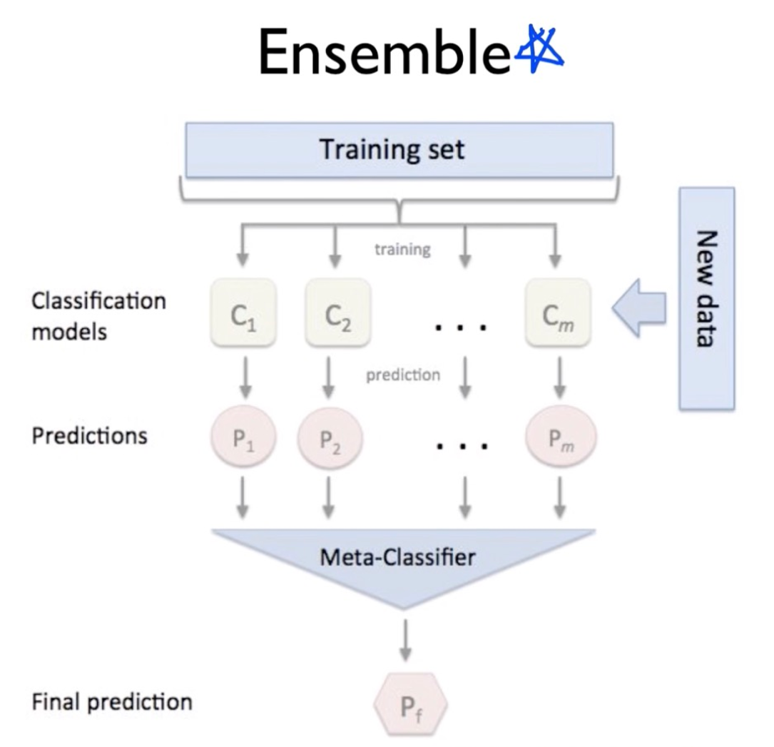
머신러닝, 딥러닝에서 앙상블은 다양한 의미를 가진다. 일반적으로 모델의 성능을 끌어 올리기 위해 독립적인 여러 모델을 모아 훈련 및 예측을 진행하는 것을 의미하는데, 훈련 데이터 셋은 별도여도 되고, 모두 같은 데이터 셋을 사용해도 상관이 없다고 한다.
(문쌤의 표현을 빌리자면, 중지를 모은다고… 명대사였다)
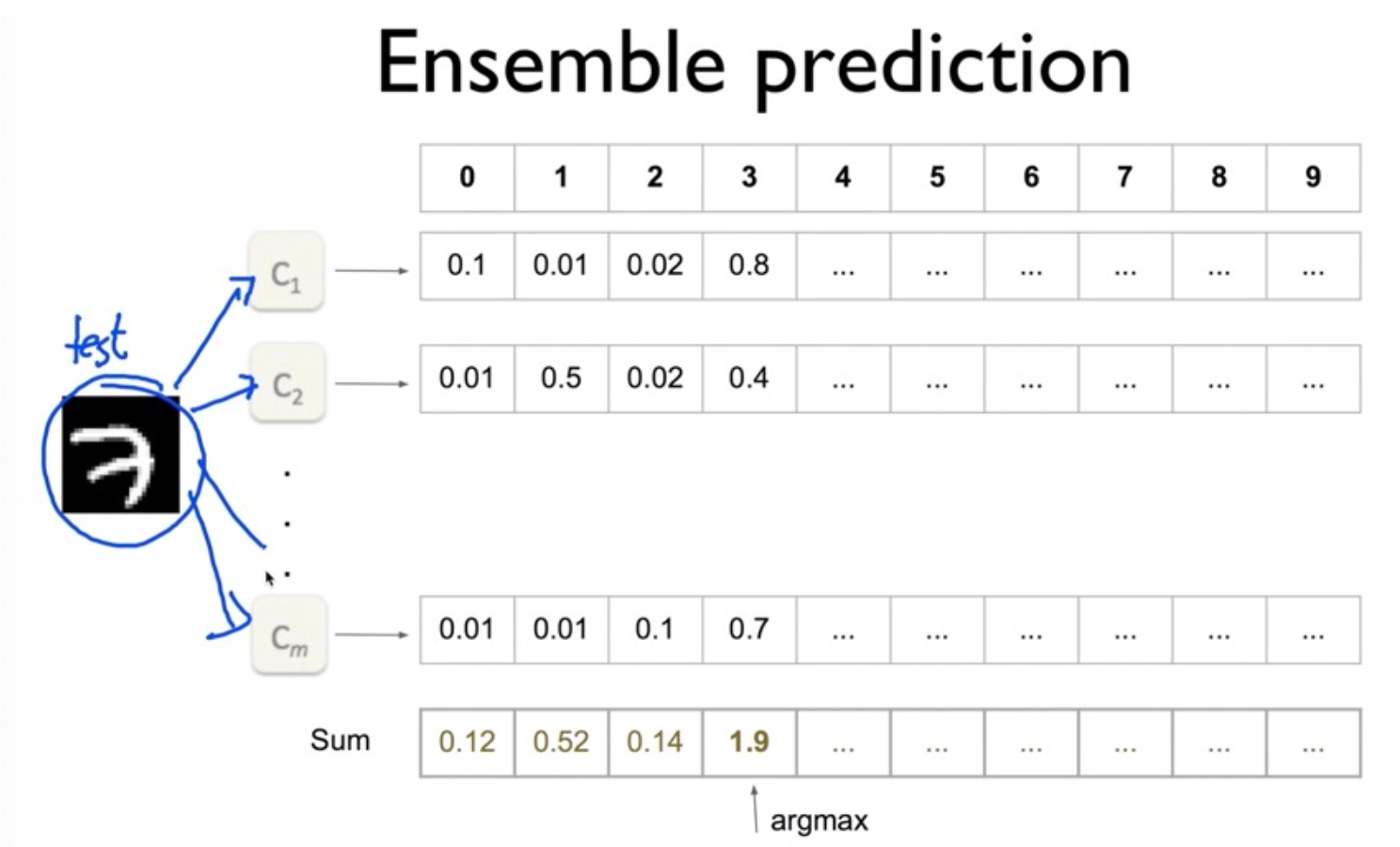
| Ensemble Concept | Ensemble Prediction |
|---|---|
 |
 |
이제 이전에 구현했던 CNN 모델을 여러 개 만들고, 각 모델의 예측 결과를 조합하는 방식으로 앙상블 기법을 구현해 본다.
Logic으로 한 번 구현하고, OOP를 사용해 동일한 내용을 객체 지향 방식으로 구현해 본다. 말하자면, CNN_1, CNN_2, … 등 여러 개의 CNN 모델을 학습시키고 예측함으로써, 하나의 CNN 모델만을 활용할 때보다 성능을 높이는 것이다.
2. 구현
2.1. Logic으로 구현하기
두 가지 방식으로 구현할 수 있다. 첫째, CNN 모델을 여러 개 만들고, 각각의 모델에서 한 번씩 학습을 진행한다. 둘째, 전체 그래프 노드들을 생성해 놓고 학습만 여러 번 진행한다.
첫 번째 방식은 매우 비효율적이기 때문에, 두 번째 방식을 사용하도록 한다.
1) 그래프 노드 생성
모델의 껍데기들을 만들어야 한다.
먼저 필요한 모듈을 불러 오고, 데이터를 준비한다.
import tensorflow as tf # tensorflow==1.15.0
import pandas as pd
import numpy as np
import matplotlib.pyplot as plt

from tensorflow.examples.tutorials.mnist import input_data
mnist = input_data.read_data_sets("./data/mnist", one_hot=True)
모델의 개수를 입력 받도록 설정하고, 그래프 노드들을 생성한다. 이제는 이전과 달리 tf.layers.conv2d 함수를 활용한다. 커널, 패딩, stride 옵션 등을 한 번에 줄 수 있어 편리하다.
# 생성할 모델의 개수
num_of_models = int(input())

# 그래프 초기화
tf.reset_default_graph()

# 변수 placeholder 설정
X = tf.placeholder(shape=[None,784], dtype=tf.float32)
y = tf.placeholder(shape=[None,10], dtype=tf.float32)
drop_rate = tf.placeholder(dtype=tf.float32)

# 입력 이미지 4차원 배열로 변환
X_img = tf.reshape(X, [-1, 28, 28, 1])

# convolution layers
L1 = tf.layers.conv2d(inputs=X_img, filters=32, kernel_size=[3,3], padding='SAME', strides=1, activation=tf.nn.relu)
L1 = tf.nn.max_pooling2d(inputs=L1, pool_size=[2,2], padding='SAME', strides=2)
L1 = tf.layers.dropout(inputs=L1, rate=drop_rate)

L2 = tf.layers.conv2d(inputs=L1, filters=64, kernel_size=[3,3], padding="SAME", strides=1, activation=tf.nn.relu)
L2 = tf.layers.max_pooling2d(inputs=L2, pool_size=[2,2], padding="SAME", strides=2)
L2 = tf.layers.dropout(inputs=L2, rate=drop_rate)

# 평면화
L2 = tf.reshape(L2, [-1, 7*7*64])

# FC layers
dense1 = tf.layers.dense(inputs=L2, units=256, activation=tf.nn.relu)
dense1 = tf.layers.dropout(inputs=dense1, rate=drop_rate)

dense2 = tf.layers.dense(inputs=dense1, units=128, activation=tf.nn.relu)
dense2 = tf.layers.dropout(inputs=dense2, rate=drop_rate)

dense3 = tf.layers.dense(inputs=dense2, units=512, activation=tf.nn.relu)
dense3 = tf.layers.dropout(inputs=dense3, rate=drop_rate)
가설, 비용 함수, 옵티마이저, 세션 등을 설정한다.
# hypothesis
H = tf.layers.dense(inputs=dense3, units=10)

# cost
cost = tf.losses.softmax_cross_entropy(Y, H)

# optimizer
train = tf.train.AdamOptimizer(learning_rate=0.001).minimize(cost)

# session
sess = tf.Session()
sess.run(tf.global_variables_initializer())
2) 학습 및 정확도 측정
각각의 모델에 대해 학습을 하고, test셋 이미지를 활용해 정확도를 측정한다. 정확도 측정을 위해 하나의 모델이 학습을 진행할 때마다 각 test 이미지에 대한 로짓 값을 구할 수 있도록 미리 NumPy의 배열을 만들어 두면 된다.
즉, 모델의 개수만큼, 테스트 셋 이미지의 각 라벨에 대한 로짓 값을 구하면 되는 것이다. 이후 로짓 값을 모두 누적하고, 이를 test셋 이미지의 라벨과 비교하여 정확도를 도출한다.
다음과 같이 구현할 수 있다.
# 예측 로짓을 기록할 배열
initial_predict = np.zeros([mnist.test.num_examples, 10])

# 학습
for i in range(num_of_models): # i번째 모델
    print(f"{i+1}번째 가설")
    num_of_epoch=30
    batch_size=100

    for step in range(num_of_epoch):
        num_of_iter = int(mnist.train.num_examples/batch_size)
        cost_val = 0
        for iter in range(num_of_iter):
            batch_X, batch_y = mnist.train.next_batch(batch_size)
            _, cost_val = sess.run([train, cost], feed_dict = {X:batch_X, y:batch_y, drop_rate=0.3})
    print(f"{i+1}번째 가설 학습이 완료되었습니다.")

    # test set 이미지에 대한 예측
    result = np.array(sess.run(H, feed_dict = {X:mnist.test.images}))

    # logit값 기록 : 각 이미지에 대해 수행.
    initial_predict += result

# test set 이미지에 대한 최종 예측값 확인
print(initial_predict)

# 정확도 측정
prediction = tf.argmax(initial_predict, 1)
is_correct = tf.equal(prediction, tf.argmax(y, 1))
accuracy = tf.reduce_mean(tf.cast(is_correct, dtype=tf.float32))
accuracy_rate = sess.run(accuracy, feed_dict = {y:mnist.test.labels, drop_rate:0})
print(f"정확도는 {accuracy_rate * 100}% 입니다.")
25번 학습한 결과의 예측 로짓 배열과 정확도를 출력하면 다음과 같다.
# 예측 결과
[[-4687.28277206 -2773.54403019 -3135.08037806 ...   461.82504082
  -3635.76250458 -2876.44646454]
 [-3064.4747963  -3136.57480812   559.18213081 ... -2139.38010025
  -2939.58929825 -3291.35899353]
 [-1837.63289261   535.95387268 -1271.67940331 ... -1310.62822533
  -1471.20205402 -1515.37879562]
 ...
 [-3922.72684097 -4249.00827026 -3603.19491386 ... -3351.75465584
  -2846.63739395 -2211.07951546]
 [-2044.20656776 -1989.31406784 -2715.41027069 ... -1875.8542366
  -1437.93685722 -1262.5892849 ]
 [-1926.148633   -2506.64439869 -2218.1466732  ... -3583.95843124
  -1665.76169205 -2345.74920845]]

# 정확도
정확도는 99.36000108718872% 입니다.
예측 로짓에 대한 softmax 함수를 적용하지 않았기 때문에, 각 라벨에 대한 예측이 0과 1 사이의 수로 도출되지 않음에 유의하자.
이전에 설계한 CNN 모델보다 정확도가 높아진 것을 확인할 수 있다.
3) 문제 : OOP 도입의 필요성
test셋에 대해 정확도를 구하는 것까지는 완료했다. 그러나, 문제는 새로운 데이터에 대해 예측을 진행할 수 없다는 것이다.
for loop을 돌면서 마지막 모델만 그래프 노드에 남아 있는 상태이기 때문에, 위에서 구현한 방법으로 예측을 진행하면, 마지막 모델을 가지고만 예측하게 된다. 과적합 등의 문제가 발생할 수 있고, 앙상블 개념에 맞지 않는다.
진정한 의미에서 앙상블 개념을 구현하기 위해서는 모든 모델이 다 남아 있어야 한다. 가설 자체(각각의 모델에서 W, b 값)를 저장할 필요가 있다. 이를 위해서는 객체지향 방식을 사용할 필요가 있다.
2.2. OOP로 구현하기
OOP로 구현하기 위해서는 다음의 사항들에 주의하자.
- 구조를 먼저 생각하자.
- class 안에 변수와 함수 덩어리를 넣어야 한다.
- class 안에 넣을 것, 밖에서 호출할 것 등을 구분해야 한다.
self의 사용에 주의하자. class 안에서 계속 사용하는 변수의 경우,self를 붙인다.
- 단계별로 객체가 생성되는지, 함수가 제대로 호출되는지 확인하며 진행하자.
이제 구조에 유의하며, OOP로 CNN 앙상블 모델을 구현해 보자.
- class 안에 정확도 구하는 부분까지 설계한다.
- list를 이용해 각 CNN 모델을 하나씩 저장하자.
- 저장한 모델들을 활용해 예측한다.
참고
만약 앙상블이 아닐 경우, class 안에 정확도 구하는 함수, 예측하는 함수 등을 모두 구현해도 된다. 다만, 지금은 앙상블을 학습하며 문제점을 해결하기 위해 OOP를 구현하는 과정이므로 정확도를 구하는 부분까지만 class 안에 정의한다.
1) Class 설계
CNN 모델 객체를 class로 정의한다. 이전과 달리, dense 함수를 사용한다. 또한, cost 함수는 softmax(logits)에 대한 cross entropy 함수로 정의한다.
# Class 설계
class CnnModel:
    # 1. 생성자
    def __init__(self, session, data):
        print("객체 생성")
        self.sess = session
        self.mnist = data
        self.build_graph() # 객체 생성 즉시 그래프를 그린다.

    # 2. 그래프 그리는 기능
    def build_graph(self):
        print("그래프 그려")

        # placeholder
        self.X = tf.placeholder(shape=[None,784], dtype=tf.float32)
        self.y = tf.placeholder(shape=[None,10], dtype=tf.float32)
        self.drop_rate = tf.placeholder(dtype=tf.float32)

        # convolution layers
        X_img = tf.reshape(self.X, [-1, 28, 28, 1])

        L1 = tf.layers.conv2d(inputs=X_img, filters=32, kernel_size=[3,3], padding='SAME', strides=1, activation=tf.nn.relu)
        L1 = tf.layers.max_pooling2d(inputs=L1, pool_size=[2,2], padding='SAME', strides=2)
        L1 = tf.layers.dropout(inputs=L1, rate=self.drop_rate)

        L2 = tf.layers.conv2d(inputs=L1, filters=64, kernel_size=[3,3], padding='SAME', strides=1, activation=tf.nn.relu)
        L2 = tf.layers.max_pooling2d(inputs=L2, pool_size=[2,2], padding='SAME', strides=2)
        L2 = tf.layers.dropout(inputs=L2, rate=self.drop_rate)

        # 평면화
        L2 = tf.reshape(L2, [-1, 7*7*64])

        # FC layers
        dense1 = tf.layers.dense(inputs=L2, units=256, activation=tf.nn.relu)
        dense1 = tf.layers.dropout(inputs=dense1, rate=self.drop_rate)

        dense2 = tf.layers.dense(inputs=dense1, units=128, activation=tf.nn.relu)
        dense2 = tf.layers.dropout(inputs=dense2, rate=self.drop_rate)

        dense3 = tf.layers.dense(inputs=dense2, units=512, activation=tf.nn.relu)
        dense3 = tf.layers.dropout(inputs=dense3, rate=self.drop_rate)

        # hypothesis
        self.H = tf.layers.dense(inputs=dense3, units=10)

        # cost
        self.cost = tf.losses.softmax_cross_entropy(self.y, self.H)

        # optimizer
        self.train = tf.train.AdamOptimizer(learning_rate=0.001).minimize(self.cost)

    # 3. 학습시키는 기능
    def train_graph(self):
        self.sess.run(tf.global_variables_initializer()) # 변수 초기화
        print("텐서플로우 그래프 학습")

        num_of_epoch = 3
        batch_size = 100

        for step in range(num_of_epoch):
            num_of_iter = int(self.mnist.train.num_examples/batch_size)
            cost_val = 0

            for iter in range(num_of_iter):
                batch_X, batch_y = self.mnist.train.next_batch(batch_size)
                _, cost_val = self.sess.run([self.train, self.cost],
                                            feed_dict={self.X : batch_X, self.y : batch_y, self.drop_rate:0.4})

            if step % 3:
                print("cost : {}".format(cost_val))

    # 4. H 로짓 값 출력 기능
    def get_Hval(self):
        print("입력한 값에 대한 H를 리턴해요!")
        return self.sess.run(self.H, feed_dict={self.X : self.mnist.test.images, self.drop_rate : 0})
모델 객체가 생성되자마자 바로 그래프 노드가 필요하므로, 그래프 그리는 기능을 생성자에 포함한다. 학습은 class 밖에서 호출하여 진행하므로, 생성자 안에 포함하지 않는다.
학습에 시간이 오래 걸리기 때문에, 학습 횟수를 3으로 지정했다.
H 로짓 값을 출력할 때, 드랍아웃을 설정하지 않음에 유의한다.
2) 모델 객체 생성
설계한 클래스로부터 여러 개의 모델을 객체로 만든다. 즉, 모델들의 틀을 만들어 놓는 과정이다. 객체 생성 시, session 변수와 data 변수를 정의하고 넘겨주어야 함을 잊지 말자.
# data load
mnist = input_data.read_data.sets("./data/mnist", one_hot=True)

# session
sess = tf.Session()

# 모델 수
num_of_model = 2

# 생성될 모델 객체 저장할 리스트
models = [CnnModel(sess, mnist) for model in range(num_of_model)]
생성된 모델 객체를 확인하면 다음과 같다.
# 모델 객체 2번 생성
객체 생성
그래프 그려
객체 생성
그래프 그려

# 모델 리스트
[<__main__.CnnModel object at 0x7f858574c7f0>, <__main__.CnnModel object at 0x7f858574c860>]
3) 모델 학습
학습시킬 때마다 다른 모델이 완성된다. 리스트에 생성된 모델 객체에 대해 class에서 정의한 train_graph 함수를 호출하면 된다.
# 모델 학습
for i in range(num_of_model):
    models[i].train_graph()
콘솔 창에 다음과 같이 cost값이 출력되는 것으로 보아, 학습이 제대로 진행되었다.
텐서플로우 그래프 학습
cost : 0.03126775100827217
텐서플로우 그래프 학습
cost : 0.11475653946399689
4) H 로짓 값 구하기
test셋 데이터에 대한 H 로짓 값을 구한다.
# 로짓값 저장할 배열
initial_predict = np.zeros([mnist.test.num_examples, 10])

# 로짓값 구하기
for i in range(num_of_model):
    initial_predict += models[i].get_Hval()
print(initial_predict)
콘솔 창에 다음과 같이 출력되고, initial_predict 값을 확인하면 다음과 같다.
입력한 값에 대한 H를 리턴해요!
입력한 값에 대한 H를 리턴해요!
[[-6.04032948  0.34726589 -0.9403764  ... 14.83251128 -5.59466042
  -0.97225238]
 [-0.1277486  -0.64623719 17.21786486 ... -6.39279358 -3.36734584
  -7.31494238]
 [-3.8862772  12.1824569  -1.60509282 ... -2.31005266 -2.47345691
  -2.32049342]
 ...
 [-7.53872459 -1.67548626 -3.11262582 ... -2.32601954 -1.1806551
  -1.2335626 ]
 [-3.01522733 -5.56961885 -7.96787756 ... -6.74841453  2.54983649
  -2.02720371]
 [-1.59091121 -4.21687557 -2.31935791 ... -8.22261503 -2.14330608
  -6.05175292]]
5) 정확도 구하기
이제 정확도를 구하면 된다. logic으로 구현할 때와 크게 다르지 않다.
# H값에서 예측값 뽑아내기
prediction = np.argmax(initial_predict, axis = 1)

# 라벨값 확인하기
actual = np.argmax(mnist.test.labels, axis = 1)

# 정확도
is_correct = np.equal(prediction, actual)
accuracy = np.mean(is_correct.astype(np.float32))
print(f"정확도는 {accuracy * 100}%입니다.")
6) 새로운 데이터에 대한 예측
이제 각각의 다른 모델 객체들이 저장되어 있으므로, 필요한 모델을 활용해 새로운 데이터에 대한 예측을 진행할 수 있다. (다만, 이 수업에서는 새로운 데이터가 있는 것은 아니므로, 그 과정은 생략한다.)
공유하기
Twitter Facebook LinkedIn

댓글남기기