
[DL] AutoEncoder_2.구현_차원 축소 2
조성현 강사님의 강의 및 강의 자료를 기반으로 합니다. Github Repo: MyUtils
Tensorflow : 2.2.0
오토 인코더 구현-차원 축소-시계열
시계열 주식 데이터를 활용해 데이터의 차원을 축소하고, 예측해 보자. 각 날짜별로 시가, 최고가, 최저가, 종가, 단기 이동평균(10일), 장기 이동평균(20일), MACD, RSI가 기록되어 있는 주가 데이터를 3개의 차원으로 축소한다. 원 데이터의 feature 개수가 많지 않아 축소하는 것이 큰 의미는 없을 것이다. 다만 LSTM 네트워크를 사용해 시계열 데이터의 차원 축소를 구현하기 위해 오토인코더를 어떻게 구성해야 하는지 초점을 맞추자. (강사님께서 미리 만들어 놓으신 MyUtil 패키지의 함수를 사용한다.)
1. 차원 축소
feature 개수를 오토인코더 네트워크를 구성해 줄인다.
# 모듈 불러오기
from tensorflow.keras.layers import Input, Dense, LSTM
from tensorflow.keras.layers import Bidirectional, Timedistributed
from tensorflow.keras.model import Model
from tensorflow.keras.optimizers import Adam
import numpy as np
import matplotlib.pyplot as plt
import pandas as pd
from MyUtil import TaFeatureSet
import pickle

# 1) 파라미터 설정
n_step = int(input('시계열 recurrent timestep 설정: '))
n_hidden = int(input('축소할 피쳐 차원 수 설정: '))
MASHORT = int(input('종가 단기이평 기간 설정: '))
MALONG = int(input('종가 장기이평 기간 설정: '))

# 2) LSTM 데이터 생성
def createData(X_data, step=n_step):
    n_feature = X_data.shape[1] # feature 수
    m = np.arange(X_data.shape[0] + 1) # 시계열 수

    # 시계열 데이터 x
    x = []
    for i in m[0:(-step-5)]:
        a = X_data[i:(i+step), :] # 20일씩 끊어서 데이터 생성
        x.append(a)
    X = np.reshape(np.array(x), (len(m[0:(-step-5)]), step, n_feature)) # 3차원 구조 변환

    # 시계열 데이터 x에 대한 5일 후 이동평균
    y = []
    for i in m[0:(-step-5)]:
        b = X_data[i+step+5-1, 4] # 5일 후 이동평균 feature 열: SHORTMA(index 4)
        y.append(b)
    Y = np.reshape(np.array(y), (len(m[0:(-step-5)]), 1))

    return X, Y

# OHLC 정규화
def normalizeOHLC(ohlc):
    m = np.mean(ohlc.mean())
    scale = np.mean(ohlc.std())

    rdf = pd.DataFrame((ohlc['open']-m) / scale) # rdf 열
    rdf['high'] = (ohlc['high']-m) / scale
    rdf['low'] = (ohlc['low']-m) / scale
    rdf['close'] = (ohlc['close']-m) / scale

    return rdf

# 데이터 로드 및 OHLC 정규화
df = pd.read_csv(f"{data_path}/069500.csv", index_col=0, parse_dates=True)[::-1]
df = df.drop(columns=['volume'], axis=1)
ndf = normalizeOHLC(df) # OHLC 정규화

# 3) 피쳐 추가 및 정규화
ndf['maShort'] = pd.DataFrame(df['close']).rolling(window=MASHORT).mean() # 단기이평 계산
ndf['maLong'] = pd.DataFrame(df['close']).rolling(window=MALONG).mean() # 장기이평 계산
ndf['macd'] = MACD(df) # MACD 계산
ndf['rsi'] = RSI(df) # RSI 계산
ndf = ndf.dropna()
ndf['maShort'] = (ndf['maShort'] - ndf['maShort'].mean()) / ndf['maShort'].std()
ndf['maLong'] = (ndf['maLong'] - ndf['maLong'].mean()) / ndf['maLong'].std()
ndf['macd'] = (ndf['macd'] - ndf['macd'].mean()) / ndf['macd'].std()
ndf['rsi'] = (ndf['rsi'] - ndf['rsi'].mean()) / ndf['rsi'].std()

# 학습 데이터 생성
data = np.array(ndf)
X_train, y_train = createData(data, n_step)

# 4) LSTM 오토인코더 모델 네트워크 설정
X_input = Input(batch_shape=(None, X_train.shape[1], X_train.shape[2])) # Input
X_encoder = Bidirectional(LSTM(n_hidden, return_sequences=True), merge_mode='sum')(X_input) # 인코더
y_decoder = Bidirectional(LSTM(n_hidden, return_sequences=True), merge_mode='sum')(X_encoder) # 디코더
y_output = TimeDistributed(Dense(X_train.shape[2]))(y_decoder) # 출력

# 5) 모델 구성 및 학습
model = Model(X_input, y_output)
print("=========== 모델 전체 구조 ===========")
print(model.summary())
print()
model_encoder = Model(X_input, X_encoder)
print("=========== 인코더 모델 구조 ===========")
print(model_encoder.summary())
print()

# 모델 학습
EPOCHS = int(input('학습 에폭 수 설정: '))
BATCH = int(input('배치 사이즈 설정: '))
model.compile(loss='mse', optimizer=Adam(lr=0.001))
hist = model.fit(X_train, X_train,
                 epochs=EPOCHS,
                 batch_size=BATCH)

# loss 시각화
plt.plot(hist.history['loss'], label='Train Loss')
plt.title('Loss Trajectory')
plt.show()

# 결과 확인
X_train_encoded = model_encoder.predict(X_train)
print(X_train_encoded.shape)
for i in range(5):
    print(X_train[i], X_train_encoded[i])
    print()
1), 2), 3) 데이터 준비
1)에서 단기 이평, 장기 이평 확인 기간을 설정하고, 3)에서 그에 맞게 피쳐를 추가해 준다. 원래 데이터에는 OHLC밖에 없다. 2)에서 LSTM 데이터를 생성할 때에는 5일 후 단기 이동평균을 예측하고자 한다. 이전에 했던 것처럼, 배치 데이터 shape에 맞게 데이터를 생성하면 된다.
4) 오토인코더 모델 생성
인코더, 디코더 모두 양방향 many-to-many LSTM 모델로 구성했다. TimeDistributed 함수를 사용해 오류를 모든 timestep에 역전파했다. merge_mode로는 sum 옵션을 사용했다.
5) 모델 구성 및 학습
전체 모델의 구성을 확인하면 다음과 같다. feature 및 시계열 기간 수가 애초에 많지 않았기 때문에, params 수가 많지 않다.
=========== 모델 전체 구조 ===========
Model: "model"
_________________________________________________________________
Layer (type)                 Output Shape              Param #
=================================================================
input_1 (InputLayer)         [(None, 20, 8)]           0
_________________________________________________________________
bidirectional (Bidirectional (None, 20, 3)             288
_________________________________________________________________
bidirectional_1 (Bidirection (None, 20, 3)             168
_________________________________________________________________
time_distributed (TimeDistri (None, 20, 8)             32
=================================================================
Total params: 488
Trainable params: 488
Non-trainable params: 0
_________________________________________________________________
None
오토인코더 모델이기 때문에, 입출력 모두 자기 자신이 나오도록 X_train을 넣어 준다. 차원이 축소된 latent feature를 확인하기 위해 인코더 부분의 모델만 구성하고, .predict 하자. 데이터의 shape이 (2362, 20, 8)에서 (2362, 20, 3)으로 그 feature가 축소된 것을 볼 수 있다. 첫 번째 데이터만 그 변화를 나타내면 다음과 같다.
[[-1.90584668 -1.83141018 -1.90711368 -1.83141018 -2.05836195 -1.75823767
   0.00271388 -0.54454236]
 [-1.85358276 -1.83426094 -1.88082335 -1.86435229 -2.06462581 -1.76773517
   0.38967395 -0.5372517 ]
 [-1.82064065 -1.72561533 -1.83552795 -1.73131685 -2.05490034 -1.77458473
   1.1058655  -0.10149927]
 [-1.73131685 -1.71864681 -1.75443968 -1.72276457 -2.03785604 -1.78127558
   1.57457442 -0.42892093]
 [-1.85896752 -1.81905689 -1.88937563 -1.81905689 -2.02140517 -1.79022177
   1.514041   -0.62360457]
 [-1.82064065 -1.75855744 -1.85611676 -1.77249449 -2.00409713 -1.79833265
   1.59319651 -0.08863674]
 [-1.77091073 -1.76964373 -1.83014318 -1.8067036  -1.97419543 -1.80659389
   1.48566798 -0.13028251]
 [-1.79023255 -1.75443968 -1.81905689 -1.78199702 -1.9451509  -1.81288379
   1.45751764  0.13797445]
 [-1.70914428 -1.68317069 -1.74493714 -1.69140622 -1.91683165 -1.81649234
   1.69369119  0.69554289]
 [-1.66669963 -1.5951139  -1.6720844  -1.63344077 -1.88877615 -1.82104479
   1.97049143  0.736402  ]
 [-1.63502453 -1.60461643 -1.65846411 -1.62520525 -1.86731419 -1.82594807
   2.09004454  1.48983144]
 [-1.57579208 -1.56343879 -1.60873419 -1.57325807 -1.83701688 -1.82844565
   2.24199636  1.51705419]
 [-1.57452508 -1.56058803 -1.5951139  -1.57864284 -1.82112645 -1.82826188
   2.21427707  1.32931348]
 [-1.57864284 -1.56058803 -1.5951139  -1.56343879 -1.8045437  -1.82867954
   2.13728377  1.24052595]
 [-1.51529263 -1.44940841 -1.51941039 -1.47949976 -1.76920234 -1.82948979
   2.24908946  1.26589752]
 [-1.52099415 -1.48646828 -1.52352816 -1.49058605 -1.7398611  -1.8300578
   2.1616766   1.40632224]
 [-1.53999921 -1.49755457 -1.53999921 -1.52922968 -1.7109814  -1.83143607
   1.86221089  0.81753024]
 [-1.52922968 -1.46587947 -1.54284997 -1.48646828 -1.68022255 -1.83343246
   1.70152203  0.92109593]
 [-1.54158297 -1.48805204 -1.56217179 -1.54570073 -1.66505741 -1.83684889
   1.30790725  1.17739644]
 [-1.53461444 -1.50452309 -1.54570073 -1.52099415 -1.65335388 -1.83743361
   1.05329261  1.11846025]]
============================================================
[[-0.3521402  -0.12966114 -1.5845938 ]
 [-0.4922347   0.07156649 -1.7783151 ]
 [-0.57715786  0.3372574  -1.8452299 ]
 [-0.83569205  0.35480547 -1.8887198 ]
 [-0.932207    0.29086986 -1.8908541 ]
 [-0.7681508   0.4179287  -1.874083  ]
 [-0.7690208   0.40564752 -1.871138  ]
 [-0.68018323  0.4614892  -1.8540821 ]
 [-0.54442424  0.6131968  -1.8389133 ]
 [-0.5900659   0.67510176 -1.8524272 ]
 [-0.42495155  0.7806265  -1.7992055 ]
 [-0.4353094   0.81122684 -1.8054175 ]
 [-0.49316406  0.7914352  -1.8022525 ]
 [-0.51114845  0.7704005  -1.7855282 ]
 [-0.53968996  0.7880661  -1.7744008 ]
 [-0.4991159   0.7909829  -1.738506  ]
 [-0.6160876   0.67463946 -1.7443626 ]
 [-0.56305873  0.6517943  -1.6941524 ]
 [-0.4137404   0.61917925 -1.5703897 ]
 [-0.31040585  0.6011925  -1.3695598 ]]
2. 이후 데이터 예측
이제 차원이 축소된 데이터를 활용해 5일 후의 단기 이동평균을 1회 예측해 보자. 원래는 차원 축소 전과 결과가 어떤지 비교해야 하지만, 연습 차원에서 1회만 예측해 보도록 한다.
# 모듈 불러 오기
from tensorflow.keras.layers import Dense, Input, LSTM
from tensorflow.keras.layers import Bidirectional, TimeDistributed
from tensorflow.keras.layers import Dropout
from tensorflow.keras.models import Model
from tensorflow.keras.optimizers import Adam
import matplotlib.pyplot as plt

# 모델 파라미터 설정
n_input = int(input('입력 피쳐 수 설정: '))
n_output = int(input('출력 피쳐 수 설정: '))
n_step = int(input('recurrent timestep 설정: '))
n_hidden = int(input('은닉 노드 수 설정: '))

# LSTM 모델 네트워크 구성
X_input = Input(batch_shape = (None, n_step, n_input))
X_lstm = Bidirectional(LSTM(n_hidden), merge_mode='concat')(X_input)
X_lstm = Dropout(0.1)(X_lstm)
y_output = Dense(n_hidden, activation='relu')(X_lstm)
y_output = Dropout(0.1)(y_output)
y_output = Dense(n_output)(y_output)

# 모델 생성
model = Model(X_input, y_output)
print("=========== 모델 전체 구조 ===========")
print(model.summary())

# 모델 학습
model.compile(loss='mse', optimizer=Adam(lr=0.001))
hist = model.fit(X_train, y_train,
                 epochs=100,
                 batch_size=300,
                 shuffle=True)
모델 구성 시 Input으로 latent feature의 수만큼을 설정해야 함에 주의한다. 모델 전체 구조를 확인하면 다음과 같다.
=========== 모델 전체 구조 ===========
Model: "model_2"
_________________________________________________________________
Layer (type)                 Output Shape              Param #
=================================================================
input_2 (InputLayer)         [(None, 20, 3)]           0
_________________________________________________________________
bidirectional_2 (Bidirection (None, 128)               34816
_________________________________________________________________
dropout (Dropout)            (None, 128)               0
_________________________________________________________________
dense_1 (Dense)              (None, 64)                8256
_________________________________________________________________
dropout_1 (Dropout)          (None, 64)                0
_________________________________________________________________
dense_2 (Dense)              (None, 1)                 65
=================================================================
Total params: 43,137
Trainable params: 43,137
Non-trainable params: 0
_________________________________________________________________
None
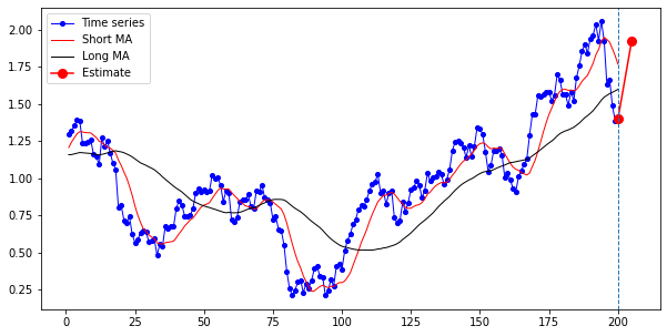
5일 후 주가 이동평균 값을 예측하면 다음과 같다. 이전 LSTM 모델에서와 마찬가지로, 입력 shape에 맞게 데이터를 바꿔 준다. 이전 200일치 데이터를 시각화하고, 이후 하루치 예측된 데이터를 시각화한다.
X_pred = np.reshape(X_train[-1], (-1, n_step, n_input))
y_pred = model.predict(X_pred)[0][0]

# 마지막 100개 데이터 plot 후 다음 값 그려 보기
last_data = np.array(df.iloc[-200:, [3, 4, 5]]) # 종가, 단기이평, 장기이평

# 원 시계열 데이터와 예측한 시계열 데이터
ax1 = np.arange(1, len(last_data) + 1)
ax2 = np.arange(len(last_data), len(last_data) + 5 + 1)
plt.figure(figsize=(10, 5))
plt.plot(ax1, last_data[:, 0], 'b-o', markersize=4, color='blue', label='Time series', linewidth=1)
plt.plot(ax1, last_data[:, 1], color='red', label='Short MA', linewidth=1)
plt.plot(ax1, last_data[:, 2], color='black', label='Long MA', linewidth=1)
plt.plot((200, 205), (last_data[-1:, 0], y_pred), 'b-o', markersize=8, color='red', label='Estimate')
plt.axvline(x=ax1[-1],  linestyle='dashed', linewidth=1)
plt.legend()
plt.show()
결과는 다음과 같다. (맞게 된 건지 모르겠다. 졸리니까 며칠 뒤에 다시 확인해 보자.)
공유하기
Twitter Facebook LinkedIn

댓글남기기